For serious projects you will need to create "package" files containing definitions of the functions that perform your calculations. Here are two ways to do it.
- Work entirely in Mathematica.
New Document -> Package
or: New Document -> Notebook; File -> New -> Package
or: File -> Open -> select previously created file
Edit the file, and to run the code click "Run Package" or "Run all code" in the top right corner of the window.
When finished, File-> Save - Use an external editor.
Here is a video showing how to develop a Mathematica program using a Notebook in parallel with a text editor.
- Summary:
- Create the package file, e.g. relaxation_solver.m, using
your favorite text editor. Then start up a Mathematica Notebook and
read in and execute the file:
<< relaxation_solver.m
Mathematica searches for this file in the directories (folders) listed in the variable $Path. To make sure Mathematica finds your file, you'll need to include in $Path the directory where the file is located. E.g., if it is in a folder math that is a subdirectory in your home directory,AppendTo[$Path, FileNameJoin[{$HomeDirectory, "math"}]] << relaxation_solver.m
In programs, you define functions using Module, and avoid using global variables as much as possible. For example, here is a function that calculates the moment of inertia of a sphere:
M$of$I$sphere[radius_,density_]=Module[{r$axial,z},      (* declare r$axial and z as local symbols, internal to the function *)
 r$axial[z_]=Sqrt[radius^2-z^2];                         (* you can define a function within a function *)
 Integrate[ Pi/2 * density * r$axial[z]^4, {z,-radius,radius}]
];

M$of$I$sphere[R,rho]                    (* use the function *)
  (8*Pi*rho*R^5)/15
All the symbols that we use temporarily inside the
module (r$axial and z in this case)
are declared at the start of the module as local variables.
This prevents interference with any other entity called z
or r$axial. We do not declare radius or
density as local because they are arguments to the
function we are defining.Within a function, you can use standard programming constructs such as for-loops, if-tests, and while-loops. When testing expressions you can use Boolean operators like
| "a and b" | a && b | |
| "a or b" | a || b | |
| "not a" | !a |
First example: testing whether a list contains a given element.
We define the function using delayed evaluation (
:=) because it cannot be evaluated until it is called with an actual list and element as arguments.
contains[list_,element_]:=Module[{i,found},    (* all variables internal to the function are declared as local *)
 i=1;          (* Loop counter *)
 found=False;  (* 'found' is a Boolean variable *)
 While[i<=Length[list] && ! found, (* Repeat the loop as long as the search has not succeeded and we haven't reached the end of the list *)
  found= (list[[i]]==element);     (* Check for a match: As in C and Python, we use == for testing the equality of two quantities *)
  i+=1;                            (* Increment the loop counter: As in C and Python, i+=1 means i=i+1*)
 ];
 found   (* returns a Boolean *)
];

contains[{4,9,2,8,1,-3}, -3]  (* Use the function we have just defined *)
  True
Second example:
counting how many times a given element appears in a list:
occurrences[list_,element_]:=Module[{i,nfound},
 nfound=0;
 For[i=1, i<=Length[list], i++,    (* As in C and Python, i++ means i=i+1 *)
  If[ list[[i]]==element, nfound+=1];
 ];
 If[nfound>0,
  Print["found ",nfound," occurrences"]
 ,(*else*)
  Print["found no occurrences"]
 ];
 nfound     (* returns number of occurrences *)
];
A substitution rule is something like x->2.5 which means
replace x with 2.5. You apply the rule to an expression using the /. operator, which can be read as
where...or
according to the rule.... For example,
2*x /. x->2.5
  5.0
x*Sqrt[x]/Cos[x] /.  x->2.5
  -4.93401
It is often convenient to apply a list of rules,
(x/y)*Tanh[x*y] /. {x->0.5, y->1.5}
   0.211716
Many of Mathematica's equation-solving routines return their results
in the form of lists of rules (or lists of lists of rules!). Note that /. is a very low priority operator, so if you want to apply a rule to part of an expression you should use parentheses to ensure that the rule gets applied in the way you intended:
( Tanh[y/x] /. {y->x^2} ) - Tanh[x]
   0
The Solve command attempts to find all solutions of an equation. For example, to find the two roots of a simple quadratic x^2 - c,
eqn = ( x^2 - c == 0 ); (* As in C and Python, we useWe see here that the Solve command returns a list of solutions. Each solution is itself a list of substitution rules, taking the form x -> EXPRESSION. To set some variable x$soln equal to one of the solutions you have to apply the corresponding list of substitution rules to the unknown variable that was in the equation (x in this case). For example: x$soln2 = x /. solution$list[[2]] in the example above.==for testing the equality of two quantities *) solution$list = Solve[ eqn, x] {{x -> -Sqrt[c]}, {x -> Sqrt[c]}} (* There are two solutions in the list *) x$soln1 = x /. solution$list[[1]] (* to get the first solution, apply the first set of rules to x *) -Sqrt[c]) x$soln2 = x /. solution$list[[2]] (* to get the second solution, apply the second set of rules to x *) Sqrt[c])
For multiple simultaneous equations with multiple unknowns, give Solve a list of equations and a list of unknowns, and as before you'll get back a list of solutions, but now each solution will be a list of several rules, one for each unknown. Here is an example, written as a function,
twovar$root[c_] = Module[{x,y,eqn$list,rules$list},   (* all variables internal to the function are declared as local *)
 eqn$list = { x^2 +y^2 == 2*c, x + y == 0};
 rules$list = Solve[ eqn$list, {x,y} ];               (* solve the two equations for x and y *)
 (* At this point, rules$list is {{x -> -Sqrt[c], y ->  Sqrt[c]}, {x -> Sqrt[c], y ->  -Sqrt[c]}} *)
 {x,y} /. rules$list[[2]]
];

twovar$root[w]     (* use the function we just defined *)
  {Sqrt[w], -Sqrt[w]}
To slice out part of a list, use the ;; construction:
list1 = {1,2,3,4,5,6,7,8,9};
list1[[4;;8]]
  {4, 5, 6, 7, 8}
The index -1 means the last element of the list, -2 means the next-to-last,
and so on:
list1[[5;;-1]]
  {5, 6, 7, 8, 9}
list1[[-4;;-1]]
  {6, 7, 8, 9}
Lists can be built using the Table function:
list2 = Table[ i, {i,1,9} ]
  {1, 2, 3, 4, 5, 6, 7, 8, 9}
To populate lists with more complicated contents, we can use the fact that
anywhere a value is required, one can put a series of statements,
separated by semicolons, that yield
that value. For example, to make a series of {x,f[x]} pairs:
xy$list = Table[x=i/5.0; y=Tanh[x]; {x,y} , {i,0,10} ]
  {{0., 0.}, {0.2, 0.197375}, {0.4, 0.379949}, {0.6, 0.53705},
   {0.8, 0.664037}, {1., 0.761594}, {1.2, 0.833655}, {1.4, 0.885352},
   {1.6, 0.921669}, {1.8, 0.946806}, {2., 0.964028}
  }
Logarithmic axes
In plots of functions, one can make one or both axes logarithmic:
LogPlot[ 1.5^x , {x,0,10} ]             (* logarithmic y axis *)
LogLinearPlot[ Tanh[x] , {x,0.01,10} ]  (* logarithmic x axis *)
LogLogPlot[ x^1.67, {x,0.01,10} ]       (* logarithmic x and y axis *)
ListsOne can plot lists of (x,y) co-ordinates instead of functions:
xylist = Table[ x=i/10.0; y=x^2; {x,y}, {i,1,10} ]  (* 10 points on the y=x^2 curve *)
  {{0.1, 0.01}, {0.2, 0.04}, {0.3, 0.09}, {0.4, 0.16}, {0.5, 0.25}, {0.6, 0.36}, {0.7, 0.49}, {0.8, 0.64}, {0.9, 0.81}, {1., 1.}}
ListPlot[xylist];
Lists can also be plotted on logarithmic axes:
  ListLogPlot[xylist];    (* y axis is a log axis *)
  ListLogLogPlot[xylist]; (* both axes are log *)
Controlling line style
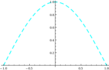
To control color, thickness, etc, use the PlotStyle option:
(* one plot style for one curve *)
Plot[ Cos[x*Pi/2], {x,-1,1},
 PlotStyle->{Cyan,Thickness[0.007],Dashing[{0.03,0.03}]}
];
 |
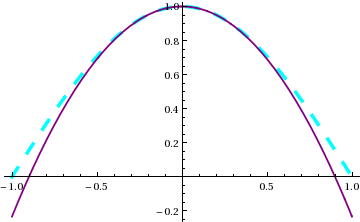
(* list of plot styles for different curves *)
Plot[ {Cos[x*Pi/2],1-x^2*Pi^2/8}, {x,-1,1}, PlotStyle->{
 {Cyan,Thickness[0.01],Dashing[{0.03,0.05}]},
 {Purple, Thickness[0.005]}
 } ];
|
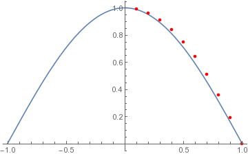
To combine two separate plots into a single plot, use the Show function. In this case, when we create plot1 and plot2 we stop them from being displayed by setting the DisplayFunction to do nothing (
Identity), and then set it back to the default ($DisplayFunction) when we combine the plots using Show:
plot1 = Plot[ Cos[x*Pi/2], {x,-1,1}, DisplayFunction->Identity ];

xylist = Table[ x=i/10; y=1-x^2; {x,y}, {i,1,10} ];
plot2 = ListPlot[xylist,PlotStyle->{Red},DisplayFunction->Identity ];

plot$12 = Show[plot1,plot2];       (* combine plot1 and plot2 on a single plot *)
Show[plot$12, DisplayFunction->$DisplayFunction]; (* show the combined plot on the screen *)
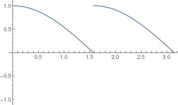
You can also use Show to combine plots that cover different ranges, by using the PlotRange option to tell it what range to cover in both x and y directions:
plot$cos = Plot[ Cos[x],{x, 0,  Pi/2}, DisplayFunction->Identity ];
plot$sin = Plot[ Sin[x],{x, Pi/2, Pi}, DisplayFunction->Identity ];
plot$both = Show[ {cos$plot,sin$plot}, PlotRange->{{0,Pi},{-1,1}}, DisplayFunction->$DisplayFunction ];  (* show the combined plot on the screen *)
As always, you can export the result to PDF, PNG, or whatever format you prefer:
Export["cos_sin_plot.pdf",plot$both]; (* create PDF file of the combined plots *)
For example, suppose we want a root of x^3 - Tanh[x]. We use FindRoot and tell it to search in the range x=0 to x=1.0:
x$rule = FindRoot[ x^3 - Tanh[x] , {x,0,1.0} ]
  {x -> 0.}
x$soln = x /. x$rule
  0.
As with Solve, the result is returned in the form of a rule,
but FindRoot returns at most one solution, which in this case
may not be what was intended: there are two roots
in the range x=0 to 1, and FindRoot found the
trivial one. Specifying a narrower initial search range helps it find the
non-trivial solution:
x$rule = FindRoot[ x^3 -Tanh[x], {x,1.0,1.2} ];
x$soln = x /. x$rule
  0.893395
Note that Mathematica will go outside the initial search range
(in this case x=1.0 to 1.2) if necessary.It is also OK to provide only one initial guessed value instead of a range.
For multiple simultaneous equations, just provide lists of expressions and variables. Here is an example, written as a function that is defined by delayed evaluation (:=) because FindRoot needs numbers to work with.
xy$solutions[x$guess_?NumericQ, y$guess_?NumericQ] := Module[{x,y,xy$rule},
 (* See the section on Type-Checking for an explanation of why the ?NumericQ patterns are needed *)
 xy$rule = FindRoot[ {x^3-Tanh[y], y - x^2}, { {x,x$guess}, {y,y$guess} } ];
 {x,y} /. xy$rule
];

xy$solutions[0.7,0.5]
  {0.853834, 0.729033}
Let's solve the time evolution equation for a classical harmonic oscillator, using the mathematica DSolve function.
eqn = ( D[theta[t],{t,2}] == -theta[t] );  (* or we could have written it as theta''[t] == -theta[t] *)
bc = {theta[0]==1, theta'[0]==0};          (* boundary conditions *)

soln$rules$list = DSolve[ {eqn, bc} , theta[t], t]
  {{theta[t] -> Cos[t]}}
theta$soln[t_] = theta[t] /. soln$rules$list[[1]]  (* there is only one solution, but we still have to specify the first solution *)
  Cos[t]
DSolve returns a list (of length 1) containing a
list of substitution rules (see Rules... above), one
for each unknown function in the differential equation.
In this case there is one unknown function theta,
so soln$rules$list[[1]] is a list containing one rule
that replaces instances of the unknown theta[t] with the
solution to the differential equation.We then applied that rule to define theta$soln to be the analytic function which solves the differential equation.
theta$soln''[t] + theta$soln[t]
  0
Let us again solve the time evolution equation for a classical harmonic oscillator, this time numerically using NDSolve,
SHO$solution[tmax_?NumericQ]:= Module[{eqn,bc,theta,t,soln$rules$list},
 (* See the section on Type-Checking for an explanation of why the ?NumericQ patterns are needed *)
 eqn = ( D[theta[t],{t,2}] == -2*theta[t] );  (* or theta''[t] == -2*theta[t] *)
 bc = {theta[0]==0.5, theta'[0]==0};          (* boundary conditions *)
 soln$rules$list = NDSolve[ {eqn, bc} , theta, {t,0,tmax}]; (* We evolve from t=0 to tmax *)
   (* At this point soln$rules$list is {{theta -> InterpolatingFunction[{{0., }}, <>]}} *)
 theta /. soln$rules$list[[1]]      (* NDSolve always gives one solution, but you still have to ask for the first solution *)
];

phi$IF = SHO$solution[3.14];  (* Try using the function we have just defined *)
(* phi$IF is now an InterpolatingFunction, which can be evaluated, plotted, etc *)
phi$IF[0]
  0.5
phi$IF[2.5]
  -0.461702
Plot[ phi$IF[tau], {tau,0,3.14}];
Like DSolve, NDSolve returns a list (of length 1)
containing a
list of substitution rules, one
for each unknown function in the differential equation.
In this case soln$rules$list[[1]] is a list containing one rule
that replaces instances of the unknown theta with the numerical
solution to the differential equation in the form of an InterpolatingFunction. To get that Interpolating Function we have to apply that rule to theta. Mathematica treats the Interpolating Function like a numerically defined function, so you can plot it, numerically integrate it, etc.
As we just saw, Mathematica expresses the solution of a differential equation as an InterpolatingFunction object. It is useful to be able to manipulate these, and to do so requires importing a special module called DifferentialEquations`InterpolatingFunctionAnatomy. With that in place, you can open up an InterpolatingFunction object and read off its properties.
fn$IF = Interpolation[ Table[ x=i/10.0; y=Sqrt[x]; {x,y}, {i,0,20}], InterpolationOrder->2]; (* Construct our own InterpolatingFunction *)
Plot[{ fn$IF[x],Sqrt[x]},{x,0,2}];   (* interpolation works well except near x=0 *)

(* Import the module that can look inside the InterpolatingFunction: *)
Needs["DifferentialEquations`InterpolatingFunctionAnatomy`"];

(* We can obtain the x limits over which the interpolating function is defined,
  allowing us to plot it even if we didn't generate it ourselves *)
{x$min,x$max} = InterpolatingFunctionDomain[fn$IF][[1]]
  {0., 2.}
Plot[ fn$IF[x], {x,x$min,x$max} ];

(* We can obtain the x-y points between which the function is interpolated *)
xvals = InterpolatingFunctionCoordinates[fn$IF][[1]]
  {0., 0.1, 0.2, 0.3, 0.4, 0.5, 0.6, 0.7, 0.8, 0.9, 1., 1.1, 1.2, 1.3, 1.4, 1.5, 1.6, 1.7, 1.8, 1.9, 2.}
yvals = InterpolatingFunctionValuesOnGrid[fn$IF]
  {0., 0.316228, 0.447214, 0.547723, 0.632456, 0.707107, 0.774597, 0.83666, 0.894427, 0.948683, 1., 1.04881, 1.09545, 1.14018, 1.18322, 1.22474, 1.26491, 1.30384, 1.34164, 1.3784, 1.41421}

(* we can find out what order polynomial is used in the interpolation *)
order = InterpolatingFunctionInterpolationOrder[fn$IF][[1]]
  2

(* we can switch the x and y data points to make a new InterpolatingFunction that is approximately the inverse of the original function *)
fn$inv$IF = Interpolation[ Transpose[ {yvals,xvals} ], InterpolationOrder->2 ];

fn$inv$IF[fn$IF[3.0]]
  2.95755 (* The inversion is approximate *)
Unexpected errors can occur if we define a function that will accept symbols as arguments, but the function then uses its arguments in numerically evaluated functions like FindRoot or NIntegrate.
The rule is: if an argument is going to be used in numerics, use a NumericQ pattern to ensure that it is a number not a symbol.
| Good: | trans$root$numeric$good[width_?NumericQ] := Module[{x}, (* NumericQ pattern ensures that 'width' is a number *) x /. FindRoot[ x^3 - Tanh[x/width]==0, {x,1} ] (* FindRoot will only work if 'width' is a number *) ]; |
| Bad: |
trans$root$numeric$bad[width_] := Module[{x},  (* No constraint on what 'width might be: it could be a symbol *)
 x /. FindRoot[ x^3 - Tanh[x/width]==0, {x,1} ]  (* FindRoot will only work if 'width' is a number *)
];
|
This function returns the root of a transcendental equation as a function of a parameter 'width' in the equation. The root cannot be found symbolically, so it has to be done numerically.
The problem with trans$root$numeric$bad is that it will allow itself to be called even when the argument that has been provided is a symbol rather than a number. Errors will occur if we later put this function into a context where Mathematica tries to call this function with a symbol as the argument. For example,
NIntegrate[ trans$root$numeric$bad[a], {a,1/2,1} ]
  FindRoot::nlnum: The function value {1. - 1. Tanh[1./a]} is not a list of numbers with dimensions {1} ...
This surprising error arises because Mathematica covertly attempts some symbolic manipulation of the integrand, which fails because the FindRoot that is hidden inside trans$root$numeric$bad fails when given a symbolic expression. To prevent this, we must define the function as shown for trans$root$numeric$good above, with a _?NumericQ pattern that tells it to only accept numbers as arguments.
If we do this, the function can be numerically integrated without error messages:
NIntegrate[ trans$root$numeric$good[a], {a,1/2,1} ]
  0.472751
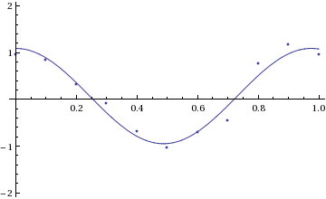
Mathematica has various fitting functions, such as Fit and FindFit, but the most powerful is NonlinearModelFit. Here is an example where we use it to fit a nonlinear function (a + b*Cos[omega*t]) to data. The three fit parameters are the vertical offset a, the amplitude b of the cosine, and the frequency omega of the cosine.
xydata = {{0., 0.951}, {0.1, 0.846}, {0.2, 0.309}, {0.3, -0.095}, {0.4, -0.694}, {0.5, -1.029}, {0.6, -0.706}, {0.7, -0.448}, {0.8, 0.768}, {0.9, 1.171}, {1., 0.963} };

nlmfit = NonlinearModelFit[ xydata, a + b*Cos[omega*t], {{a,0.2}, {b,1.0}, {omega,5}}, t];  (* we give an initial guess for each parameter *)
NonlinearModelFit can be rather sensitive to the initial guesses for the parameter values. If the fit is successful then
nlmfit is now a FittedModel object, which superficially behaves like the best-fit function to the data, but also contains a lot of information about the fit.
Normal[nlmfit]   (* shows the best fit function *)
  0.0707912 + 1.01908 Cos[6.44376 t]
nlmfit[0.75]     (* evaluate the best fit function at t=0.75 *)
  0.193222
(* We can make a plot of the data and the fit: *)
plot$data=ListPlot[xydata,DisplayFunction->Identity];
plot$fit=Plot[nlmfit[t],{t,0,1},DisplayFunction->Identity];
Show[{plot$fit,plot$data},PlotRange->{-2,2},DisplayFunction->$DisplayFunction];
We can also extract information about the fit:
nlmfit["BestFitParameters"]
  {a -> 0.0707912, b -> 1.01908, omega -> 6.44376}
nlmfit["ParameterErrors"]
  {0.0621924, 0.0790336, 0.162831}  (* a is not significantly different from 0, but b and omega are *)
nlmfit["ParameterTable"]
             Estimate    Standard Error   t-Statistic   P-Value
     a       0.0707912   0.0621924        1.13826       0.287949
     b       1.01908     0.0790336        12.8943       1.23746*^-6
     omega   6.44376     0.162831         39.5732       1.82829*^-10

nlmfit["AdjustedRSquared"]
   0.940382
We can obtain many other diagnostics and properties of the fit, including an ANOVA table. See the Mathematica documentation for full details.